Chapter 15.10 - Curtailment of bars in frames

In the previous section we saw the lengths of bars and areas of bars that have to be embedded at a simple support and at a continuous support. These requirements are given in the sub clause (a) of 26.2.3.3.

Now we will see the next sub clause: cl.26.2.3.3(b). This clause is related to framed structures. We have seen a framed building in the presentation given at the beginning of chapter 9 on 'Flanged sections'. Such framed structures are assumed to consist of two dimensional frames arranged in two mutually perpendicular directions. A two dimensional frame can be seen in the slide no.7 of the presentation. These frames are acted upon by the Live loads and Dead loads which generally act in a 'vertical direction'. The frames are analysed for these loads, and the effects such as Bending moments, Shear forces, Torsions etc., at various points are determined. But some times, Wind and/or Earth quake loads also act on the structure. These loads act in a 'horizontal direction'. So they are called 'lateral loads'. Then the frames of the structure has to be analysed for these lateral loads also. Such frames are called 'lateral load resisting frames'. They have to made much more stronger to resist these additional lateral loads. The fig.15.46 below shows the horizontal forces acting on such a frame.

Fig.15.46

Horizontal forces acting on a frame

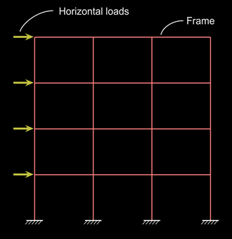
If all the loads are 'vertical', the bottom bars will be experiencing zero forces at the supports. But if there is a combination of horizontal loads and vertical loads, stress reversal can occur. In such cases, the bottom bars may experience tensile or compressive forces near the supports. (More details can be obtained from text books on structural analysis of frames.) As the bars experience forces near supports, they have to be given more anchorage. 

We have seen how the anchorage is ensured for bottom bars at simple supports and continuous supports.  We have seen the three parameters related to such simple supports in the previous section:

(i) Length of the embedment. 

(ii) quantity of the bars which are embedded.

(iii) Position of the bars which are embedded.

Here, for lateral load resisting frames, (ii) and (iii) are the same. [(ii) is same as that at a continuous support, which is equal to A_st/4]. 

• But (i) which gives the 'length' is changed from L_d/3 to L_d. That means, we have give the full development length (unique value), and not one third of it. Such an increase will give more anchorage.

We will now see the methods by which this can be achieved at various points in a lateral load resisting frame. The following figs. shows the extensions to be given to the bottom bars when the beam is part of a lateral load resisting frame.

Fig.15.47

Extension into an intermediate Column

From the above fig., we can see that at an intermediate column, there is enough space to extend the bars. So L_d can be easily provided.

Fig.15.48

Extension at an end support with standard 90^o bend

At the end support, we can not extend bars freely. So we may have to provide a bend. The above fig. shows the case when a standard 90^o bend is given. The anchorage value of the portion from B to D is 8Φ. So the total anchorage value is equal to A'B + 8Φ, and this should be greater than or equal to L_d.

Fig.15.49

Extension beyond the bend

Here the anchorage value of the portion from B to D is 8Φ. So the total anchorage value is equal to A'B + 8Φ + DE, and this should be greater than or equal to L_d.

It must be noted that for seismic design of structures, more detailed rules have to be followed by referring the related codes.

Next clause is 26.2.3.3 (c). We have already discussed about it in detail here.

---

So we have seen most of the details about the bottom bars. In the discussions, we saw the extension that has to be given at the supports for the 'continuing bars'. We also saw the extension that has to be given to the 'curtailed bars'. (15.4). Thus we are now in a position to design the curtailment and give the necessary extensions for the bottom bars of various members. After determining the layout and position of the bottom bars using the principles that we saw so far, the check for 'development length' has to be done. The following fig.15.50 can be used to perform this check for the bottom bars in general.

Fig.15.50

Check for development length

There are two types of bars to be considered: 

• Those which are curtailed at some point. The top layer bars in the above fig. is an example for this. They are curtailed at section XX.

• Those which are not curtailed at any point. They continue uninterrupted into the supports. The bottom layer bars in the above fig. is an example of this.

Let XX be the section at which the curtailment is actually done. That is., XX is the section which is determined by making the necessary modifications to the theoretical cut-off point. We know that all the bars (both curtailed and continuing) at the section CL will be under maximum tensile stress. To keep the curtailed bars from 'contracting', the length available is the distance between CL and XX. So this distance must be greater than or equal to L_d (unique value). This length should be available for each of the curtailed bars.

Similarly, at the section XX, the continuing bars will be under maximum tensile stress. So to keep them from 'contracting', each of these bars should have a length which is greater than or equal to L_d . This length should be available on the left side. It may be noted that for the continuing bars, the check for L_d need to be made from the theoretical cut-off section only, and so a greater length is available to qualify as L_d, than if checked from XX.

In the above fig., the mid span section CL is shown, and also the section XX at which curtailment is done is also shown. XX is to the left of CL. So the fig. is a part elevation of the 'left side of a span'. 

As the bars try to contract from both ends, we must provide the necessary L_d  on both sides of the sections being considered. In the above fig., we can see that the bottom bars have a greater distance on the right side of the theoretical cut-off section, as this section is near the left support. But after fixing up the layout of all the bars, we must check and confirm that the required L_d is actually available on both sides of all important sections.

   

If the bars satisfies this check also, the layout and positions of the bottom bars can be finalised.

---

Now we will see the details about the top bars which resist the hogging moment. The requirements regarding these are given in the cl.26.2.3.4 of the code. In this clause, there are two parameters that we have to satisfy. (i) length and (ii) quantity. We will now see the details about each of them:

(i) Length: We know that, after the point of inflection, the moment change from hogging to sagging. So top bars are not required beyond the point of inflection. But the code does not allow us to stop the top bars exactly at that point. It requires us to extend the top bars beyond the point of inflection, to a distance which is greater than the largest of the following:

(1) effective depth d

(2) 12 times the diameter of bar ie., 12Φ

(3) 1⁄16  of clear span.

(ii) Quantity: The continuing bars that goes beyond the point of inflection should have a total area of  A_st ⁄ 3 . where A_st is the maximum area of the top steel at the support.

These two requirements can be discussed in detail with the help of the fig.15.51 below:

Fig.15.51

Curtailment of Top bars

Near the support, an area A_st1 of steel is provided for the top bars in the above fig. Out of these, some bars are curtailed. We can see that the curtailed bars are extended beyond the theoretical point of curtailment, for a distance of L_a. This is based on 15.4 which we derived earlier. But the present clause that we are discussing, is about the continuing bars. The code does not allow us to stop the continuing bars at the point of inflection. But instead, they are extended even beyond the point of inflection by a distance which is greater than or equal to the largest of

(1) effective depth d

(2) 12 times the diameter of bar ie., 12Φ

(3) 1⁄16  of clear span

It can also be seen than the area of these continuing bars is shown to be greater than or equal to A_st1 ⁄ 3.

If we are using a moment envelope, p₀^h should be used as the point of inflection. All the other procedures remain the same. This is shown in the fig.15.52 below:

Fig.15.52

Moment envelope for curtailment of top bars

The arrangements shown in the above can be used also for the framed structures. So these figs. can be used for framed structures just by changing the support from ‘masonry type’ to ‘concrete column’. A 'continuing column' can also be shown if the beam belongs to an intermediate floor. For the top most floor, there will not be a continuing column. All the other details remain the same as in the above figs. The modified figs. for framed structure are shown below:

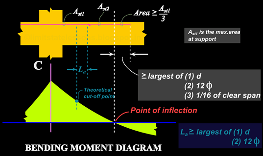
Fig.15.53
Curtailment of top bars (intermediate support in framed structure)

Fig.15.54

Moment envelope for curtailment of top bars (intermediate support in framed structure)

Now, the above two figs.15.53 and 54 can be used to show the curtailment of top bars at the 'end support of a frame'. For this we have to make some modifications only at the support. The other details remain the same. This is shown in the figs. below:

Fig.15.55

Curtailment of top bars (end support in framed structure)

Fig.15.56

Moment envelope for curtailment of top bars (end support in framed structure)

From the above two figs., we can see that the bars have to be given a standard 90^o bend and should be extended into the column, for obtaining the necessary development length. The anchorage obtained for each bar is equal to A’B + 8Φ + DE. And this anchorage must be greater than or equal to L_d. All other details about the curtailment of bars are the same as that at an intermediate support.

One more detail that we have to see about top bars is when they are provided at a simple support. We will discuss about it in the next section.

PREVIOUS       CONTENTS       NEXT                                          

Copyright©2016 limitstatelessons.blogspot.com- All Rights Reserved

Chapter 15.4 - Internal forces in an RCC beam

In the previous sections we completed the discussion on the methods to determine the theoretical cut-off points. We saw the exact method as well as the approximate method. Both the methods give us 'theoretical points'. As mentioned earlier, the bars should not be stopped at these theoretical points. They must be continued further. This means that the 'actual' cut-off points will be different from the 'theoretical' ones. 

One of the obvious reasons for not accepting the theoretical points can be stated as follows: We have used the BM diagrams for calculating the points. But these diagrams can undergo unexpected changes. These unexpected changes may occur due to changes in loads, changes in positions of Live loads, sinking of supports etc., So the points obtained from BM diagrams cannot be relied upon. In this and the following sections, we will explore more reasons for continuing the bars beyond the theoretical points, and also 'how much' further we have to take the bars.

Consider a simply supported beam. When the factored load is applied on the beam, flexural cracks (‘flexural cracks’ means the cracks formed due to the bending of the beam) will be first appearing in the midspan region as shown in the fig.15.19 below:

Fig.15.19
Flexural cracks appearing at midspan region

Also, the midspan section will reach the ultimate state. That is., the steel at the midspan section will yield, and the concrete strain at that section will become 0.002. While the midspan section is undergoing these changes, other sections which are at some distance away from the midspan will still be in a safe condition. This is because, these other sections have a 'capacity' (we measure this ‘capacity’ in terms of the ultimate moment of resistance, MuR) which is greater than the applied factored bending moment at these sections.

But when we do 'curtailment of bars', the section or sections at which the curtailment is done, will also become critical sections. This is because, the applied factored bending moment at a section where curtailment is done, will be comparable to the capacity of the section. At such sections flexural cracks will begin to form as shown in the fig.15.20 below:

Fig.15.20
Flexural cracks appearing at a section XX at which curtailment is done

These flexural cracks may develop into diagonal tension cracks as shown in the fig.15.21 below. The possibility of formation of such diagonal cracks is high if heavy shear force is present near the section at which curtailment is done.

Fig.15.21
Flexural cracks developed into a diagonal tension crack

We will now analyse the forces in this cracked beam. For this, we will first look at an ordinary un-cracked beam shown in fig.15.22 below.

Fig.15.22
Simply supported beam with a factored udl of wu kN/m

From the basic lessons of strength of materials, we know how to calculate the applied bending moment at any section XX, at a distance 'x' from either support. We draw a free body diagram of the portion on the right of section XX. This is shown in the fig.15.23 below:

Fig.15.23
Free body diagram of the portion to the right of XX

• The moment at XX, due to the reaction R_B is equal to R_B x (anti-clock wise). 
• The moment at XX due to the applied load w_u is equal to (w_u x² )/2 (clock wise) 
• So the net factored moment at XX is given by:

M_u,x = R_B x  – (w_u x² )/2 

This equation will give us the applied factored bending moment at any section. Now we can look into the internal forces as shown in the fig.15.24 below:

Fig.15.24
Equilibrium of internal forces

• The compressive force C_u acts at the centroid of the 'concrete area above the neutral axis'.
• The tensile force T_u acts at the centroid of the steel area.
• These two forces are equal in magnitude but opposite in direction. So they form a couple. The magnitude of this couple is equal to T_u z . It is also equal to C_u z . Here, z is the lever arm.
• This couple resists the applied factored bending moment M_u,x.

So now we know the details about the internal forces. We can use the same procedure for analysing the internal forces in the cracked beam shown in fig.15.19 above. We will discuss about it in the next section.

PREVIOUS       CONTENTS       NEXT                                          

Copyright©2016 limitstatelessons.blogspot.com - All Rights Reserved

Chapter 15.3 - Approximate method for theoretical points of curtailment

In the previous sections we saw the method of finding the theoretical points. We used the method of solving the equation of Bending moment. In this section we will discuss about another method to determine the theoretical cut-off points. 

For this we will first discuss about a special phenomenon that occur at the sections where curtailments are done: We have seen a beam in which there is a total of 8 bars at midspan, and some of these bars were curtailed at various sections. Figs.15.7, 15.8 and 15.9 showed the theoretical sections of curtailment.  

Now let us look at the depth of neutral axis xu which were noted down earlier at each of the sections CL, LL, MM and NN.  • xu,CL = 250.67, • xu,LL = 205.55, • xu,MM = 160.43, • xu,NN = 80.21. We have also noted down the effective depth d at these sections. From these, we can make a table which gives the lever arm z at each of these sections. The table so formed is given below:

Name of Section	d (mm)	xu (mm)	z = d- 0.416xu
CL	533.3	250.67	429.02
LL	545.439	205.55	459.93
MM	554	160.43	487.26
NN	554	80.21	520.63

The next step is to calculate a particular ratio at each of the section where curtailment is made: The ratio of 'z at midspan' to 'z at the section'. These are calculated below:
zCL / zLL = 429.02 / 459.93 = 0.9328
zCL / zMM = 429.02 / 487.26 = 0.8805
zCL / zNN = 429.02 / 520.63 = 0.8240
All the values are close to '1'. So they can be taken approximately to be equal to ‘1’.

When the beam is loaded to the ultimate state,
• the midspan section (section CL in our example ) will reach the ultimate state. 
• The sections at which curtailments are made ( sections LL, MM, and NN in our example ) will also reach the ultimate state. 

In such a situation, the following phenomenon will occur:

---

The ratio: [ z at midspan / z at a section where curtailment is done ] can be approximately taken to be equal to '1'. In other words, the lever arm at all the sections where curtailment is done will be approximately equal. They will all be approximately equal to the lever arm at midspan.

---

Now, we know that the ultimate moment of resistance MuR at any section is given by MuR = 0.87 fy Ast  z . So we can write:
MuR,CL =0.87 fy Ast,CL  zCL   and   MuR,LL =0.87 fy Ast,LL  zLL 

Taking ratios, we will get
MuR,CL    / MuR,LL   = [ Ast,CL  / Ast,LL] x [ zCL / zLL  ]

But by the special phenomenon that we saw above, [ zCL / zLL  ] =1. 
So we can write:
MuR,CL    / MuR,LL   = [ Ast,CL  / Ast,LL]

We can rearrange this equation as :
• MuR,LL   = MuR,CL  x [ Ast,LL  / Ast,CL]
Similarly we can write:
• MuR,MM   = MuR,CL  x [ Ast,MM  / Ast,CL]  and
• MuR,NN   = MuR,CL  x [ Ast,NN  / Ast,CL]

We can get a general form from the above three equations. For this, let us assign the name ‘XX’ to denote any section at which curtailment is made. Then we can write the general form as:
Eq.15.3:
MuR,XX   = MuR,CL  x [ Ast,XX  / Ast,CL]
   
Ast,XX  is the area of steel remaining in the section after curtailment is made. So, if we intend to curtail a particular number of bars of a particular diameter, we can calculate the area  Ast,XX  which remains after curtailment. So MuR,XX is the only unknown in Eq.15.3.

This gives us an easy method to calculate the MuR at a section where curtailment is made. When we do a curtailment, the remaining bars which continue the journey will be less. As a result, the MuR which remains will also be less. We can calculate this remaining MuR using Eq.15.3. There is no need to do a 'detailed analysis of the section' with the remaining bars and the new value of d.

When MuR at a section is determined, the only step remaining is to find the position at which this much factored bending moment is applied on the beam. We have seen earlier that, this step is done by solving for x in the equation for BM.

So this is an approximate method to calculate the theoretical cut-off points in the beam. Let us now use this method to find the theoretical cut-off points in our beam. We can show the results in a table as given below:

Name of Section	Ast,XX (mm2)	Ast,XX  / Ast,CL	MuR,XX	Distance from support A (mm)
CL	1256.637	_	194.65	_
L1L1	1030.442	0.8200	159.61	1.5358
M1M1	804.248	0.6400	124.57	1.0517
N1N1	402.124	0.3200	62.29	0.4570

Note that the sections are renamed as L1L1, M1M1 and N1N1 , because their positions are slightly different from those of LL, MM and NN that we obtained using the exact method.

Sample calculation:
Let us take section M1M1
• Ast remaining after curtailment at section M1M1 = 804.248 mm²  
• Ratio  [Ast,XX  / Ast,CL] at this section = 804.248 / 1256.637 = 0.6400
• This ratio multiplied by the MuR at midspan will give the MuR at M1M1 (Eq.15.2)
So MuR,M1M1 = 0.6400 x 194.65 = 124.57 kNm

In this ‘approximate method of calculating theoretical cut-off points’, MuR at the midspan (MuR,CL in our example) is the only MuR that we have to calculate using the exact method of analysis that we learned in chapter 3

• Now we can use Eq.15.2 to determine the distance of M1M1 from the support A.
Eq.15.2:
M_u,XX = 150 x – (1.5 x 40 x²)/2 where x is the distance of the section from the support A.
• We can put M_u,XX = 124.57 in the above equation, and obtain x = 1.0517 (the same value in the above table)  and it's symmetric counterpart 3.9483 m. 

The fig. showing all the sections is given below:

Fig.15.18
Final theoretical sections using approximate method

Here is a comparison of the results from the two methods:
Distance from support A:
• Exact Method: LL =1.7609, MM =1.2616, NN =0.5686 m
• Approximate method: L1L1 =1.5358, M1M1 =1.0517, N1N1 =0.4570 m

So we have seen two methods to determine the theoretical curtailment points. In the next section, we will discuss about the modifications that have to be made to the theoretical cut-off points.

PREVIOUS       CONTENTS       NEXT                                          

Copyright©2016 limitstatelessons.blogspot.com - All Rights Reserved

Chapter 15.2 - Curtailment at points of inflection

In the previous section we saw the method of finding the theoretical point of curtailment at more than one section along the length of the beam. In this section we will see the method for the top bars which resist the hogging moment at an intermediate support of a continuous beam.

In fact the method is the same: Find the M_uR obtained from the remaining bars, and put it in the equation to obtain 'x'. So we will discuss only the general scheme adopted for the top bars. This is shown in the fig.15.9 below:

Fig.15.11
Curtailment of top bars

• The first curtailment is given to the bars in the bottom most layer (when counted from the top) among the top bars. When they are curtailed, the steel that remains is A_st2. 
• The second curtailment is given to the second bottom most layer. After this curtailment, the steel that remains is A_st3. 

When we follow this pattern, greater quantities of steel are available at the regions nearer to the support. This indeed must be the case because, stresses are greater near the supports as far as the 'top bars for hogging moments' are concerned.

Another aspect to note is the position of 'points of inflection'. These are the points where the bending moment changes sign. The hogging nature of the bending moment at the support continues upto the points of inflection. So we have to provide top steel upto the point of inflection. Similarly, the sagging nature of the bending moment at the midspan region also continues upto the points of inflection. So we have to provide the bottom steel upto these points. But we can follow the principles of curtailment, and progressively reduce the quantity of steel at the sections near the points of inflection.

We will now discuss another aspect of the point of inflection. In continuous beams, the maximum bending moment at any section will depend upon the position of the loads along the spans. The DL will be present at all times, and it's position will not change. But the LL will change position. In order to find the maximum bending moment at a section, we have to place the LL in those positions that give maximum bending moment at that section, and then analyse the whole continuous beam. This topic is dealt with in 'influence lines' in Structural analysis classes. 

We had a basic discussion about it in the second section of chapter 7, 'Analysis of a continuous beam'. Let us consider the solved example of a continuous beam ABCDE given in that chapter. We do not require the bending moments or final results obtained in that example. We are interested only in the pattern of loading that we adopted for that beam. This pattern was shown in fig.7.19 and 7.20. 

Let us consider the support C, and the span CD. We want 
• the maximum hogging moment at support C and 
• the maximum sagging moment in the span CD. 
For obtaining the maximum possible hogging moment at support C, we must place the LL on the adjacent spans BC and CD, and also on alternate spans. But after filling up BC and CD, there are no alternate spans. So we will filled up BC and CD with LL, and then analysed the whole beam. The resulting BM diagram is shown below in fig.15.12:

Fig.15.12
Maximum hogging moment at support C

But this BM diagram is prepared xxx exclusively for the hogging moment at support C. That is., only the hogging moment values at the support C should be obtained from this diagram. So we will remove the unwanted parts to obtain the fig.15.13 shown below:

Fig.15.13
Diagram with unwanted values removed

Now we will look at the span CD. For maximum sagging moment in this span, the LL should be placed on CD and on alternate spans. So we placed it on CD and on the first span AB. The resulting BM diagram is shown in the fig.15.14 below:

Fig.15.14
Maximum sagging moment in span CD

But this BM diagram is prepared exclusively for the sagging moment in span CD. That is., only the sagging moment values in span CD should be obtained from this diagram. [For this particular beam ABCDE, the above loading arrangement for the maximum sagging moment in CD is same as the loading arrangement for the maximum sagging moment in AB also. But we are not considering AB in our present discussion]. So we will remove the unwanted parts to obtain the fig.15.13 shown below:

Fig.15.15
Diagram with unwanted values removed

The figs.15.15 and 15.13 gives the required values. So we can combine the two figs. as shown below:

Fig.15.16
Required values shown in a single diagram.

The above fig.15.16 gives the maximum values of the hogging moment at support C and the sagging moment in span CD. By using the same procedure, we can fill up the remaining supports and spans in the fig. Then, from that single fig., we can obtain the maximum values at any section along the length of ABCDE. Such a fig. is called the 'moment envelope'. Now let us take a closer look at the fig.15.14. This is shown in the fig.15.17 below:

Fig.15.17
Details of the moment envelope at support C and span CD and the points of inflection

We can see that the point of zero moment in the hogging moment envelope which is marked as p₀^h is different from p₀^s the point of zero moment in the sagging moment envelope. This is a situation that we often see while analysing continuous beams and continuous one-way slabs.

• The top steel bars should be provided for the hogging moment in the region shown in orange colour in the above fig.15.17. This steel should be available upto the points where the orange graph meets the horizontal axis, which are the points of inflection. In fact, as we will soon see in later sections, the bars should be continued even beyond the points of inflection.

• The bottom steel bars should be provided for the sagging moment in the region shown in yellow colour in the above fig.15.17. This steel should be available upto the points where the yellow graph meets the horizontal axis, which are the points of inflection. In this case also, we will soon see in later sections that, the bars should be continued even beyond the points of inflection.

• So the points of inflection play a major role in the final layout of bars. But these points of inflection for the sagging and hogging moments may not coincide. That is., we cannot expect a 'continuity' at the points of inflection as we saw in the fig.15.11 earlier in this section. The meeting point with the horizontal axis may be different for sagging and hogging moments, just as p₀^h and p₀^s in the fig.15.17. This happens when the different positions of LL are considered. This non-coincidence should be considered, and exact positions of various points of inflection should be determined (from the moment envelope) so as to provide a satisfactory lay out of bars.

In the next section, we will discuss another method to determine the theoretical cut-off points.

PREVIOUS       CONTENTS       NEXT                                          

Copyright©2016 limitstatelessons.blogspot.com - All Rights Reserved