Chapter 2 - Analysis of Sections by Working Stress Method

Analysis of SectionsHere we will analyze sections of structural members which are subjected to bending (flexure). Structural members like beams and slabs are subjected to bending. Some other members like columns, walls etc., are also some times subjected to bending due to eccentric loading, lateral pressure etc.,

A structural designer have to deal with the following two types of problems:

(1) Analysis problems
When dealing with an analysis problem, the following details will be given:
● Complete cross sectional dimensions of the member
● Details of reinforcing steel
● Properties of the materials

Based on those given details, the following should be determined:
● Stresses in the materials
● Deflections, crack widths etc.,
● The ultimate bending moment or load that the member can resist

(2) Design problems
For this, the following details will be given:
● The ultimate bending moment or load that the member should resist
● Allowable stresses in the materials

Based on those given details, the following should be determined:
● Complete cross sectional dimensions of the member
● Details of reinforcing steel and required properties of the materials.

Analysis of Beams:
Beam is a commonly used structural element. It may exist independently in a structure as in a simple brick masonry car porch where it is provided above the entrance in the front. It may also exist as the part of a structural frame work with lots of beams, columns and slabs as in the case of multi storeyed buildings.

Usually a beam has to resist bending moments and shear forces. In some cases a twisting moment may exist. There may also be an axial force acting on the beam. This axial force may be tensile or compressive. But often, in the case of beams, this force will not give rise to high stresses and so it is neglected.

Theory of bending:
Reinforced concrete is not a homogeneous material. It is a composite material consisting of concrete and steel. We will first discuss the theory of bending for a homogeneous material.

The most important assumption in the theory of bending is that the plane cross sections taken normal to the longitudinal axis of the beam remain plane even after bending. (This assumption is not valid for Deep beams). Another point that we must consider here is that, when a beam bends due to a sagging moment, the fibres below the neutral axis are in tension and the fibres above are in compression. ( The reverse happens in hogging moments as in cantilevers). With this knowledge and the above assumption about the plane sections, the following point can be deducted:

● The strain in any fibre is proportional to the distance of the fibre from the neutral axis. As the distance increases, the strain also increases. In fig 2.1, the green coloured graph is obtained by plotting the strains along the X axis. The values of strains have opposite signs in the regions above and below the neutral axis. This is because above the neutral axis, the strains are compressive and below the neutral axis, they are tensile. We can see that among all the fibres in the compression zone, the top most fibre is situated at the maximum distance y_c,max    from the neutral axis, and here, the compressive stress has a maximum value of f_c,max. The compressive strain is also maximum here. Similarly,among all the fibres in the tension zone, the bottom most fibre is situated at the maximum distance y_t,max from the neutral axis, and here, the tensile stress has a maximum value of f_t,max  and the tensile strain is also maximum. When the distance from the neutral axis decreases, the stress and strain also decreases linearly, as shown by the blue and green graphs.

Fig.2.1
Stress and strain distribution in a homogeneous section

We can derive some useful equations from this diagram. For that, we first find the areas of the two triangles above and below the neutral axis in the stress diagram.

The basic bending equation is:

Where
M = Bending moment at the section
I = Moment of inertia of the section
E = Modulus of Elasticity of the material
R = Radius of curvature of the neutral layer of the beam
f = stress in the fibre
y = distance of the fibre from the neutral axis of the beam

From the above we get
 

and
 

Thus we obtained the base of each of the triangles in the stress diagram. Now, the altitudes are already known:
y_t,max for the lower triangle and  y_c,max for the upper triangle.

So We get the area of the upper triangle as (1/2) x Base x Altitude =
 

Similarly, the area of the lower triangle is

We have used 2-dimensional figs. for the calculations. But the stress diagrams are in fact, stress blocks, and they have volume. This is shown in the 3-dimensional view given below:

Fig.2.2
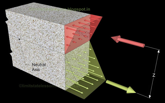
Three dimensional view of stress distribution

We know the area of the triangles. If we multiply this area by the width of the beam we will get the volume of the stress block. Volume of the compressive stress block is the total compressive force, and the volume of the tensile stress block is the total tensile force.

So total compressive force C at the section is given by:

Eq.2.1
  

and total tensile force T at the section is given by:

Eq.2.2

The total compression C acts at the centroid of the 'area above neutral axis'. The total tension T acts at the centroid of the 'area below neutral axis'. For the section to be in equilibrium, the condition C=T should be satisfied.

The Resisting moment developed at the section is given by:

Eq.2.3
M = Cz  = TzSince C = TWhere z is the 'lever arm' or the distance between the two centroids.
This M is equal to the moment applied by the external load at this section.

It may be noted that the neutral axis of a section passes through the centre of gravity or centroid of the section. It does not depend on the external load applied on the beam. If the external load increases or decreases, the change that is happening in the beam is that the force experienced by the fibres increases or decreases but the position of the neutral axis remains the same. For a beam of homogeneous material, the position of the neutral axis can be changed only by changing the dimensions of the cross section. Thus for a homogeneous beam of rectangular cross section, the position of neutral axis can be changed only by changing the width or height of the cross section. In other words, a homogeneous beam of particular cross section have a definite position of neutral axis.

Analysis of  composite Sections

The analysis described above is not suitable for non homogeneous or composite materials. Composite materials are made up of two or more materials. eg: Reinforced concrete which is made up of two materials, concrete and steel. In such cases the theory has to be modified. Fig 2.3 below shows the representation of a composite material

Fig.2.3
Representation of a Composite material

The two materials, Material 1 and Material 2  should be bonded together and should act as an integral unit without any slip at their interface. If this condition is satisfied, the strain in material 1 situated at a distance y from the neutral axis will be same as the strain in the surrounding material 2, at the same distance y from the neutral axis. So the graph showing the strains will be same for both the materials as shown in fig 2.4. (But the stresses will be different because, stress depends on the property of the material)

Fig.2.4
Stress and Strain distribution for a composite Material

In the above fig.2.4, the stresses are plotted along the X direction to a suitable scale.

The stresses can be calculated using the hookes law, which states that

Let
f_1y = Stress in a layer in Material 1, situated at a distance y from the Neutral axis
ε_y = Strain at this layer
E₁ = Young's modulus of Material 1
f_2y = Stress in a layer in Material 2, situated at a distance y from the Neutral axis
ε_y = Strain at this layer (Note that strain at this distance y  is same for both the materials, as there is no slip between the materials)
E₂ = Young's modulus of Material 2
From Eq 2.4 above, we get

and

 

From the above, it follows that

Which is same as

 

The ratio  E₂ / E₁ is denoted by m, and is called modular ratio

So we get
Eq.2.4m = E₂ / E₁

Eq.2.5
f_2y = m f_1y

We can remove Material 2 from this composite material, and replace it with Material 1. Then the composite material will once again become a homogeneous material. We must replace the Material 2 in such a way that the strength of the section of the resulting homogeneous material is same as that of the composite material that we were having. We must find the quantity of Material 1 required to achieve this.

Transformed Section:The fig 2.5 given below represents a section which is completely made up of Material 1.

Fig.2.5Representation of a Transformed section

We can see that Material 2 which was colored yellow in the previous fig 2.3, has been replaced by Material 1. But the width has been changed to b₃ and the depth has been changed to d₃, giving an area A_m3 = b₃d₃

So we started with a composite beam. We have replaced Material 2 in that composite beam with an area A_m3 of  Material 1. When this change is made, the resultant force in the beam should remain unaltered. In other words, when loaded, the new beam should give the same effect as the old composite beam.

● First let us consider fig 2.4. An infinitesimal area in Material 2 is marked off. The distance of this small region from the neutral axis is y● The area of this small region da₂  is given by da₂ = 2(b₂ / 2)d_y =  b₂d_y ● The tensile stress in this small region is f_2y 

The resultant force df₂ in this small region can be obtained by the equation:  Force = Stress x Area.

So we get
Eq.2.6.
df₂ = f_2y x da₂ 

Now we again consider the basic bending equation:

From this it follows that:

Eq.2.7

Substituting 2.7 in 2.6, we get

Total force F₂ in the Material 2 is given by summing the forces in all the infinitesimal regions. Thus:

But

Where y₂ = Distance of the center of gravity of Material 2 from the NA, and
A_m2 = Total area of Material 2

Thus we get
Eq.2.8

Similarly from fig 2.5, we can show that
Eq.2.9

Where F₃ = Total force in the newly placed Material 1
y₃ = Distance of the centroid of the newly placed Material 1 from the NA
A_m3 = b₃d₃ = Total area of the newly placed Material 1

R remains the same in both the cases because of the following reason: When we make a new beam with Material 1 only, we want it to give the same effect as the composite beam. So, when loaded, the radius R should be the same.

So we want F₂ = F₃ .
So equating Eqs.2.8 and 2.9 we get

But from 2.4, we have m = E₂ / E₁   So we get
Eq.2.10

We can simplify the above Eq.2.10 further. For this, we have to arrange the area A_m3 in the new beam, in a particular way. Fig 2.6 below shows both the sections.

Fig.2.6
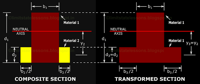
Composite section and Transformed section

In the fig, the height d₃ of the Material 1 on the sides of the transformed section is kept same as that of Material 2 in the composite section. The area is adjusted by changing only the width. When only the width is changed, the vertical distance y₃  of the centroid from the NA remains unchanged at y₂ . Thus y₂ = y₃ . Substituting this in 2.10, we get Eq.2.11
A_m3 = mA_m2  

So from the initial composite material, we can remove all the area A_m2 of Material 2 and replace it with an area mA_m2 .of Material 1 in such a way that , and centroidal distance of both A_m2 and mA_m2 from the NA are the same.

Now we can apply the above principles to Reinforced concrete which is a composite material made of Concrete and Steel.

Transformed section of a Reinforced concrete Beam:
In the working stress method (WSM) of analysis of reinforced beams, we transform the given section into an equivalent concrete section by removing the area of steel A_st and replacing it by an area of concrete equal to m A_st  We know that m = E₂ / E₁ . The subscript ‘2’ denotes that material of the composite section, which is replaced by the original material. For reinforced concrete beam, steel is the material which is being removed, and concrete is the orginal material. So m for reinforced concrete beam is given by: E_s / E_cWhere E_s = Elastic modulus of Steel and,
E_c = Elastic modulus of Concrete
The elastic modulus of steel is a constant. It can be taken as E_s = 200 kN/mm²

But that of concrete depends upon long term effects like creep. So the code gives us a formula for determining the modular ratio in the case of reinforced concrete.

Eq.2.12

(Clause B 1.3(d) of Annex B of the code)
where σ_cbc  is the permissible compressive strength of concrete in bending. It's value can be obtained from Table 21 of the code. Note that these are the permissible values upto which compression can be applied to concrete, when the concrete is subjected to bending. As in the case of a horizontal beam in which the concrete above the NA will be subjected to compression, due to the bending of the beam. It is different from the condition where the concrete is subjected to direct compression, as in the case of a column.

The following Table 2-1 gives the values of σ_cbc and m for the different grades of concrete:

We can do a sample calculation with a random value of concrete grade. Let us take M35. From table 21, the value of σ_cbc for this concrete grade is 11.5 N/mm² . So m = 280 / (3 x 11.5) = 8.11

We have seen earlier that to convert a reinforced concrete section into a transformed section, we remove the entire steel A_st  from the section and add extra concrete, and the area of this extra concrete is m A_st . The following fig. 2.7 explains the process in detail:

Fig.2.7
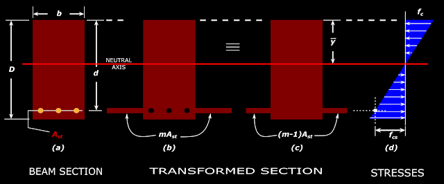
Reinforced concrete section and it’s Transformed section

In the above fig.2.7, fig (a) shows the beam section. In fig(b), all the steel has been removed and extra concrete of area m A_st  has been added. In this fig., hollow regions are present where the steel was previously placed. Also note that the new concrete is placed at the same level of steel. This is to ensure that the vertical distance of the centroids of steel and the newly placed concrete are the same. In fig (c), the hollow regions has been filled with concrete. The hollow regions have an area of A_st . So that much can be reduced from the extra concrete on the sides. So the area of the extra concrete on the sides becomes m A_st  - A_st = (m-1)A_{st .} Fig (d) shows the stress distribution in the transformed section. The stress in concrete at the level of steel (denoted as f_cs ) can be easily obtained by using the 'principles of similar triangles'.  Knowing f_cs  , we can calculate the stress in steel f_st by using Eq 2.5 , by which, the stress in Material 2 (steel) is m times the stress in Material 1 (concrete). So we get:

Eq.2.13
f_st  = mf_cs

In the above fig.2.7, two vertical dimensions are marked: D and d. D is the total depth of the beam section. d is the distance of the centroid of the steel reinforcing bars from the top most compression fibre of the beam section. It is known as the ‘effective depth’ of the beam.

Now we will try to understand the behaviour of a newly constructed reinforced concrete beam. If the load is applied for the first time on the newly constructed beam, and this load is increased gradually from zero, the bottom most concrete fibres, which are in tension, will crack for the first time, when the tensile stress in them reaches a particular value. This value of the tensile stress is called the modulus of rupture and is denoted by f_cr . The code (cl 6.2.2) gives the following empirical formula for calculating f_cr .

Eq.2.14
  

We know that the basic bending equation is

From this equation we can get the moment at first crack or the Cracking moment

Eq.2.15

Where M_cr  is the cracking moment,
I_T is the moment of inertia of the transformed section and
y_t is the distance of the extreme tension fibre from the NA.
f_cr  is calculated from Eq.2.14

Following is the link to a solved example which shows the application of the topics that we discussed above :
Solved example 2-1

PREVIOUS                                 CONTENTS                                 NEXT

            Copyright©2014 limitstatelessons.blogspot.com - All Rights Reserved

Basic design concepts in Limit State Method

First we will have a brief discussion about the limit state method. A limit state is a state of impending failure. Beyond this state, the structure will not be safe or serviceable.

Safety factorsSafety factors can be explained as follows:A structure should satisfy the condition that The resistance it can offer is always greater than or equal to the effects due to design loads.This condition can be represented by the equation:

1.1

Φ R_n ≥ γS_n

where

R_n = Nominal or characteristic value of resistance R
S_n = Nominal or characteristic value of load effect S
Φ = resistance factor
γ = load factor

Nominal or characteristic value of R is given by the code. For example,if we choose to use Fe 415 steel for a concrete member, we take it’s value of R given by the code. Similarly, if we choose to use M20 concrete, we get the R value from the code.

Characteristic strength of steel is denoted as f_y
and
Characteristic strength of concrete is denoted as f_ck

characteristic load is defined as The load that has a 95 per cent probability of not being exceeded during the life of the structure.

The above definition of ‘characteristic load’ involves some statistical calculations. But in the absence of statistical data about loads, the characteristic values of loads can be taken from the following codes:

Type of Load	Relevant code
Dead Load	IS 875 (Part 1-3)
Live Load	”
Wind Load	”
Seismic Load	IS 1893 (Part 1):2002

It is possible that the value R_n is not calculated accurately due to the uncertainties in material strength, dimensions, theoretical assumptions etc., So, to be on the safer side, we have to take a smaller value than R_n  Thus Φ will be less than unity.

Similarly there will be uncertainties about S_n . There can be overloading during some occasions. So, to be on the safer side, we have to take a larger value than S_n  . Thus γ will be greater than unity.

Partial safety factorsThe code uses the partial safety factor system:
In this system, the safety factor for resistance, ie., Φ   in 1.1, is separated into two ' Partial safety factors '.
• For concrete it is γ_c• For steel it is γ_s   

To get the resistance offered by concrete, γc  is applied to f_ck as (0.67 fck)/γ_c 
To get the resistance offered by  steel, γs  is applied to f_y as f_y/γ_s

In the case of concrete, the quantity 0.67 is coming in due to the following reason:
f_ck  is obtained by the experimental results in the lab. But the actual strength of concrete in a real structure will be less than what is obtained in the lab. This actual strength is taken as 0.67f_ck

We have seen earlier that Φ is less than unity. Now we see that γ_c and γ_s  into which Φ is separated appear in the denominator. But as we will soon see, their values given by the code are greater than unity. Thus by applying them in the denominator, we get the same effect as using a safety factor whose value is less than unity.

Similarly, the safety factor for load, ie., γ in 1.1 is separated into three partial safety factors:
• For Dead Load (DL), it is γ_D• For Live Load (LL), it is γ_L• For Wind Load OR Earthquake Load, it is γ_Q

(Only one of Wind or Earthquake Load is considered at a time. The probability that the earthquake and extreme wind will occur at the same time is taken to be negligible.)

• To get the DL, γ_D is applied to DL as γ_D x DL• To get the LL, γ_L is applied to LL as γ_L x LL• To get the Wind or Earthquake load QL, γ_Q is applied to QL as γ_Q x QL

The above safety factors which are multiplied to the loads are all greater than one. So when multiplied, they will give a greater load. This will result in more safety.
But for γ_D , the value is taken as one in some cases. Examples of such cases are:
• When stability against overturning or sliding is considered.
• When reversal of stresses is considered when dead load is combined with Wind load or Earthquake load.

Values to be used for the Partial safety factors

We have seen the various partial safety factors and the methods to apply them. Now we shall see the actual values of the partial safety factors that we must use while designing a concrete structure. For this we must first know two types of limit states:

• Ultimate limit states and
• Serviceability limit states

• Ultimate limit state is a condition specified by the code. If the structure reaches this stage, the code assumes that the failure of the structure is impending. The structure may start to slide, overturn, collapse or buckle etc.,
• Serviceability limit state is also a condition specified by the code. If the structure reaches this stage, the code assumes that the structure is beginning to cause discomfort to the occupants and/or the structure is beginning to malfunction. This may be in the form of excessive deflection, crack widths, vibration, leakage etc.,

A structure should be designed in such a way that ‘ultimate limit states’ will not be reached. And then, the final design should be checked for ‘serviceability limit states’.

Now we look at the values to be taken for the partial safety factors:

FOR THE MATERIALS CONCRETE AND STEEL,

For ultimate limit states:

• γ_c = 1.5
• γ_s = 1.15

A higher value is given for concrete because it's qualities are more variable than steel

For serviceability limit states:

• γ_c = 1.0
• γ_s = 1.0

Here we notice that, for serviceability limit states, a value of 1.0 is given. This is because if we assume a lower strength for materials by using higher partial safety factors, we will get higher deflections, crack widths etc., We want to know the actual deflections and crack widths so that we can ensure that such a state is not reached. But in the case of ultimate limit states, we want to ensure that the ultimate state is not reached even when a lower material strength is assumed. So we give values 1.5 and 1.15 (note that these values greater than unity are applied in the denominator, thus reducing the final values).

Here we notice that, for serviceability limit states, a value of 1.0 is given. This is because if we assume a lower strength for materials by using higher partial safety factors, we will get higher deflections, crackwidths etc., We want to know the actual deflections and crack widths so that we can ensure that such a state is not reached. But in the case of ultimate limit states, we want to ensure that the ultimate state is not reached even when a lower material strength is assumed. So we give values 1.5 and 1.15 (note that these values greater than unity are applied in the denominator, thus reducing the final values).

FOR LOADS,For ultimate limit states:
The following three different combinations of loads have to be calculated and the maximum value from among the three has to be taken.

Combination 1:
• γ_D = 1.5
• γ_L = 1.5
Giving Ultimate load (UL) = 1.5(DL + LL)

Combination 2:
• γ_D = 1.5
• γ_Q = 1.5
Giving UL = 1.5(DL + QL)

OR

• γ_D= 0.9
• γ_Q = 1.5
Giving UL = 0.9 DL + 1.5 QL
(0.9 is to be used for DL when the stability against overturning or stress reversal is critical)

Combination 3:
• γ_D = 1.2
• γ_L = 1.2
• γ_Q = 1.2
Giving UL = 1.2(DL + LL + QL)
(A lower value of 1.2 is given in this combination because it is assumed that all the loads will not act at the same time at their peak values)

Thus for the ultimate limit state, we see that the safety factors for loads are greater than 1.0, unless it is for special conditions. This is because we want to ensure that the limit state is not reached even at higher loads.

For Serviceability limit states:
The following three different combinations of loads have to be calculated and the maximum value from among the three has to be taken.

Combination 1:
• γ_D = 1.0
• γ_L = 1.0
Giving Serviceability load SL = 1.0(DL + LL)

Combination 2:
• γ_D = 1.0
• γ_Q = 1.0
Giving SL = 1.0(DL + QL)

Combination 3:
• γ_D = 1.0
• γ_L =  0.8
• γ_Q = 0.8
Giving SL = 1.0 DL + 0.8 LL + 0.8 QL
(A lower value of 0.8 is being used because, when LL  and QL are combined, it is improbable that both will reach their peak values at the same time)

All the above values are given in Table 18 of IS 456.

So now we know the exact values that must be used for the various partial safety factors. In the case of loads, we get the ‘Characteristic values’ of the loads from the code, and then apply the appropriate partial safety factors. But for the materials, steel and concrete, the application is not so ‘direct’. Some calculations are involved. Let us see the case of concrete first:

Curve showing the relationship between the stress and strain in concrete:

Fig 21 in section 38.1 of the code shows the relation ship between stress and strain in concrete. Strain is plotted along the X axis, and Stress is plotted along the Y axis. The top most curve is plotted using the values obtained by doing tests in the lab. But we have seen that these values are multiplied by 0.67 to get the values in a real structure. So, the curve corresponding to 0.67f_ck is the characteristic curve. From this curve, the following information can be obtained:

• when the strain increases, the stress also increases parabolically in the initial stage
• This increase continues upto a point when the strain reaches 0.002. The stress has increased to a value of 0.67f_ck• After this point the stress remains constant even if strain is increased.
• The strain can increase only upto an ultimate value of 0.0035. That is., when the strain is 0.0035, the code assumes that concrete has reached the ultimate state (the state of impending failure).

When we design a structure, we need to know the strength of concrete, which is obtained after applying the partial safety factor. So this partial safety factor is applied to the characteristic curve, and thus the bottom most curve is obtained. Thus 0.67f_ck becomes equal to (0.67/1.5)f_ck = 0.447f_ck. From this bottom most curve, we can obtain the design values.

If we know the equation of this design curve, we can find the value of stress developed in concrete for a particular value of strain. The equation consists of two parts. One for the parabolic portion and the other for the straight line portion. These are as follows:

Where fc = stress, and ε = strain

We will see the application of this curve in subsequent chapters.

Curve showing the relationship between the stress and strain in steel:

As in the case of concrete, in the case of steel also, we get the design values from the code. Fig 23 in section 38.1 of the code shows the relation ship between stress and strain in steel. Fig 23A is for cold worked bars (Fe415 and Fe500). 23B is for mild steel (Fe250).

Curve for mild steel:
From this curve, the following information can be obtained:

• When the strain increases, the stress also increases linearly in the initial stage
• This increase continues upto a point when the stress reaches a value of f_y . The strain at this point is f_y/E_s . The behavior of steel upto this point is linear elastic. That is if we remove the load, steel will regain its original length
• This point is called the yield point. And this point is well defined for mild steel.
• Beyond this point, when the strain increases, the stress remains constant.

The design curve is obtained by dividing every stress value by the partial safety factor for steel, 1.15. This is same as multiplying by (1/1.15) = 0.87 .The values thus obtained are plotted to get the lower curve.

Curve for cold worked bars:
From this curve, the following information can be obtained:

• when the strain increases, the stress also increases linearly in the initial stage
• There is no specific yeild point
• The linear elastic behavior continues upto a point where stress is equal to 0.8f_y
• After this point, the material is elastic but not linear. That is, if we remove the load, it will not fully regain it's orginal length. This behaviour continues upto a point where stress is equal to f_y . At this point, if we remove the load, there will be a residual strain of 0.002
• Beyond this point, when the strain increases, the stress remains constant.
• The design curve is obtained by dividing every stress value by the partial safety factor for steel, 1.15. This is same as multiplying by (1/1.15) = 0.87 .This is shown by the lower curve.
• The design curve for Fe 415 and Fe 500 are similar. The value of f_y  has to be changed from 415 to 500.
• We can obtain any values from the straight line portions. But in the non linear portions, it is not easy. The non linear portion is approximated as small linear segments. The code gives the end points of these small linear segments. Any point on these segments, other than the end points should be calculated using linear interpolation. The following table gives the coordinates of the end points:

Table for Fe415:

Strain	Stress (N/mm2)	Calculation
0.000	0.00
0.00144	288.7	(415 x 0.80)/1.15
0.00163	306.7	(415 x 0.85)/1.15
0.00192	324.8	(415 x 0.90)/1.15
0.00241	342.8	(415 x 0.95)/1.15
0.00276	351.8	(415 x 0.975)/1.15
≥ 0.00380	360.9	(415 x 1.00)/1.15

Table for Fe500:

Strain	Stress (N/mm2)	Calculation
0.000	0.00
0.00174	347.8	(500 x 0.80)/1.15
0.00195	369.6	(500 x 0.85)/1.15
0.00226	391.3	(500 x 0.90)/1.15
0.00277	413.0	(500 x 0.95)/1.15
0.00312	423.9	(500 x 0.975)/1.15
≥ 0.00417	434.8	(500 x 1.00)/1.15

We will see more details about the above calculations and the application of these curves in subsequent chapters. In the next chapter we will see some basic details about the analysis of sections by Working stress method.

CONTENTS   NEXT

Copyright©2014 limitstatelessons.blogspot.com- All Rights Reserved