Chapter 16 (cont..12)

The following solved example illustrates the design of a transverse stair.

Solved example 16.3

The reinforcement details according to the above solved example is shown in the figs.16.64 and 16.65 given below:

Fig.16.64
Sectional elevation of transverse stair

Fig.16.65
Section XX

We will now discuss the various features of the above two figs:
The main bars are given as the bottom most layer. The distributor bars are given as the second layer from the bottom. This arrangement will give maximum possible effective depth ‘d’ for the section. From the section XX, we can see that the main bars are given two 90^o bends at both the ends. This will give a 'hook' like arrangement at both ends. The top portion of these 'hooks' will act as the steel required for resisting any possible hogging moment at the supports. The length required for this top steel is 0.15l, where l is the effective span of the waist slab. But the area required for this top steel is only half of that at the mid span. So, as shown in the inset, only alternate bars are given these hooks.

The distributor bars are of mild steel. So the symbol Φ is given to denote them.

In the above example, only a part plan (shown in the fig.16.65 below) of the stair was given along with the problem data.

Fig.16.65
Problem data of solved example 16.3

This is because, this small portion is sufficient for defining the problem of this type of a transverse stair. Some times this stair may have a landing also as shown below.

Fig.16.66
Landing in a transverse stair

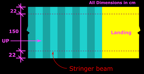
In this case also the sloping portion can be analysed and designed by the same procedure, and the landing can be analysed and designed as a simply supported one-way slab.

Stairs cantilevering from the side of a beam:

The following fig.16.67 shows the part view of a stair.

Fig.16.67
View of a cantilever stair

It is projecting from the side of a wall. The wall is shown in a finished state. So we cannot see more details. The fig. below shows the view before the plastering is applied to the wall.

Fig.16.68
View of a stair cantilevering from a stringer beam

We can see that the stair is projecting from the side of a beam, which is concealed inside the wall. In actual construction, the beam (which frames into columns) and the waist slab will be cast first, and after curing and removal of form works, the masonry wall will be constructed above and below the beam. The elevation and section are shown in the figs. below:

Fig.16.69
Part elevation view of cantilever stairs

Fig.16.70
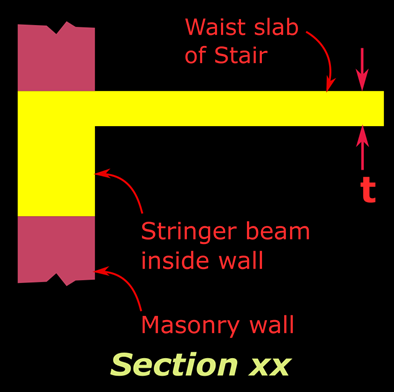
Section XX

The waist slab bends in a direction perpendicular to the direction of travel of the pedestrians, and so it is a transverse stair. The load calculation procedure is the same as that for the transverse stair supported on two stringer beams. So we can use the same Eq.16.25. The line diagram for the analysis will be as shown below:

Fig.16.80
Line diagram for cantilever stairs

The effective span l of the cantilever (cl.22.2.c) is the length of the cantilever up to the face of the support plus half the effective depth. For initial proportioning, we can assume the thickness of waist slab to be clear length of cantilever/10 . However, this should be finalized only after the complete design and doing the various checks.

In the next section, we will see a solved example of the above type of stairs.

PREVIOUS      CONTENTS      NEXT

             Copyright ©2015 limitstatelessons.blogspot.com - All Rights Reserved

Chapter 12 - Analysis of Doubly reinforced beams

In the previous section, we completed the discussion on design of a doubly reinforced beam section. In this section we will discuss the analysis. When we are given a doubly reinforced beam section for analysis, we have to find the depth of the neutral axis x_u , and the ultimate moment of resistance M_uR.

We know that when we analyse the section using the Limit State Method, we are calculating the forces in the section at the point of impending failure. The concrete at the extreme compression fibre will be about to crush. And also, if it is an under reinforced section, the steel in the tension zone would have yielded.

So now we are going to find the forces in a doubly reinforced section, at the above mentioned point of impending failure. We can base our discussions on the fig.12.1 given below:

Fig.12.1
Stresses, strains and forces

The above fig. shows all the stresses and forces at the ultimate state. We will now see the details of each component:

The depth of NA is denoted as x_u. It's value can be less than or greater than x_u,max, depending on the quantities of steel. It is one of our aims to calculate this x_u of the given beam section.

We have derived the expression for ε_sc in the previous chapter. We used the triangles above the NA in the strain diagram. We have the same strain diagram here also. The only difference is that x_u,max is now changed to x_u. So from Eq.11.1, we get:

Eq.12.1:

When we know ε_sc, we can calculate the stress f_sc in A_sc. But here we cannot use the table 11.1 because, the values in it correspond to the condition of x_u = x_u,max. Here we are having x_u, which may be having a value higher or lower than x_u,max. So we have to use the original tables for calculating f_sc.

The net compressive force in steel is obtained as:
C_us = (f_sc - 0.447f_ck) A_sc
The compressive force in concrete C_uc = 0.362f_ckbx_u 

So the total compressive force is given by:
C_u = 0.362f_ckbx_u  + (f_sc - 0.447f_ck) A_sc

The total tensile force is given by T_u = f_st A_st
equating the above two, we get 

0.362f_ckbx_u  + (f_sc - 0.447f_ck) A_sc = f_st A_st

From this we get
Eq.12.2

But from Eq.12.1, we can see that f_sc depends on x_u. So the above Eq.12.2 will not give a closed form solution. We have to use strain compatibility method.

Another point to note is that, f_st also depend on x_u. If the tension steel has not yielded at ultimate state, we cannot take f_st as equal to 0.87f_y. So for such sections also, we will have to use strain compatibility method. We will discuss the details of the method when we do a solved example.

It may be noted that the above Eq.12.2 will give a closed form solution if both the tension steel and compression steel have yielded. Because, then f_sc and f_st will be having a constant value of 0.87f_y 

Once we determine x_u, we can calculate M_uR, the ultimate moment of resistance of the doubly reinforced section. For this we will use the compressive forces. We have two compressive forces:

• C_u = 0.362f_ckbx_u. Lever arm of this force = d - 0.416x_u. So the contribution from this force = 0.362f_ckbx_u (d - 0.416x_u).
• C_us = (f_sc - 0.447f_ck) A_sc.   Lever arm of this force = d-d'. So the contribution from this force = (f_sc - 0.447f_ck) A_sc (d-d') 

Sum of the above contributions will be the M_uR. So we get:
Eq.12.3: M_uR = 0.362f_ckbx_u(d - 0.416x_u) + ( f_sc - 0.447f_ck) A_sc(d-d')

Under reinforced or Over reinforced Doubly reinforced sections

In the case of singly reinforced sections, we have seen the details of 'balanced sections'. We discussed it based on the fig.3.26. This fig. is shown again below:

Fig.3.26
Stresses and strains in singly reinforced balanced sections

From the strain diagram in this fig., we saw that x_u,Bal, (which is same as x_u,max) is the particular depth of NA at which the strain in tension steel is equal to ε*_st, the yield strain. If in a beam section, x_u is less than x_u,max, the strain ε_st will be greater than ε*_st. Then it is an under reinforced section. If x_u is greater than x_u,max, ε_st will be less than ε*_st. That means the steel will not yield at ultimate state, and it is an over reinforced section.

We can extend the above discussion to Doubly reinforced sections also. As the plane sections remain plane after bending (Details here), the strain diagram for a doubly reinforced section will also be a straight line similar the strain diagram in the above fig. Thus the ε_st of 'tension steel' in a doubly reinforced section will be greater than ε*_st if x_u is less than x_u,max. It will be less than ε*_st if x_u is greater than x_u,max. 

So we can say that while designing a doubly reinforced section, just as in the case of a singly reinforced section, we must ensure that x_u is less than x_u,max. So that, if over loading occurs, and the beam fails, the failure will be a tension failure.

In the next three sections we will see analysis examples based on the above discussions. Links to these sections are given below.

• Solved example 12.1  • Solved example 12.2  • Solved example 12.3 (over reinforced)  

After the above solved examples, a comparison between 'Under reinforced and Over reinforced' doubly reinforced beam sections is given here. 


PREVIOUS

NEXT

                                                         

            Copyright ©2015 limitstatelessons.blogspot.com - All Rights Reserved

Chapter 8 - Design examples of continuous slabs and beams

In the previous chapter we completed the analysis of the continuous slabs and beams. In this chapter we will discuss the design of continuous beams and continuous one way slabs. 

We will consider the design of continuous slabs first. For this, the first step is to setup a preliminary depth for the slab. This is for calculating the self wt. But for continuous slabs and beams, this is all the more important (unless we are using moment coefficients) because, only with the knowledge of the dimensions of cross section, we can do the 'detailed structural analysis'.

We have already seen (in the chapter 6: design of simply supported one-way slabs) that the 'control of deflection' is the criterion for deciding the depth in the case of slabs. We have derived the expressions  which will enable us to use this criterion in the case of one-way slabs: 

6.1: (l/d)_actual  ≤  20 x 1.25 ⇒ (l/d)_actual  ≤  25. So d that we actually provide in the final slab should be greater than or equal to l/25. This is for simply supported slabs.

6.2: (l/d)_actual  ≤  26 x 1.25 ⇒ (l/d)_actual  ≤  32.5. So d that we actually provide in the final slab should be greater than or equal to l/32.5.≈ l/32 . This is for continuous one-way slabs.

So using 6.2, we can easily fix up a preliminary depth for the continuous slab. But we have to consider a few points before we use this expression 6.2.:

In continuous systems, the end spans will be subjected to greater sagging moment than the interior spans. So we have to use the properties of end spans for fixing up the depth. (The depth so derived from the end span is provided for all the spans. This is for uniformity). But the end span is not 'perfectly continuous'. It is continuous only at it's interior support. At the end support, it is discontinuous or simply supported. So we cannot use the value '26'. The solution for this problem is to use the average of simply supported condition and continuous condition. That is., average of 20 and 26, which is equal to 23. Thus we get l/d basic = 23.  Thus for the end span we get:

8.1: (l/d)_actual  ≤  23 x 1.25 ⇒ (l/d)_actual  ≤  28.75. So d that we actually provide in the final slab should be greater than or equal to l/28.75.≈ l/29 . This is for end spans in continuous one-way slabs.

From the above expression, what we get is the effective depth d. To this we must add C_c and half of Ф to get the total depth D. Ф can be assumed to be equal to 10mm. 

We must do all the design checks to ensure that the final section is adequate. If the section is found to be inadequate, the whole process should be repeated with improved dimensions.

After fixing the preliminary depth, we can start the design process. The design process is same as that for a simply supported slab that we saw earlier in chapter 6: We designed it as a beam of width 1000 mm and total depth D. First we calculated d required. Then we compared it with the d obtained from the preliminary dimensions. If the required value was less, we proceeded to find the steel required to resist the sagging BM at midspan. Here, in the case of continuous one-way slabs also, we have to do the same. But we have to do this for each span. That is., we have to calculate the steel required to resist the sagging BM at the midspan of each span. Plus, we have to do this for the hogging BM at each of the supports also.

After obtaining the steel at all midspans and supports, we arrange the bars in such a way that the maximum and minimum spacing requirements between the bars are satisfied. We have to design the distribution steel also. Then we do the final checks like area of minimum steel required, check for p_t,lim, check for deflection etc., These steps will become more clear when we see an actual solved example:

Solved example 8.1:
We will do the design of the continuous slab, of which we did the structural analysis in the previous chapter 7. We have obtained the BM and SF at all the important points. We will use the results obtained by using the 'method of coefficients' fig.7.14 and 7.15. Those results are reproduced in the table 8.1 below:

Table 8.1:

	BM
Span AB	28.60
Supp. B	-29.76
Span BC	17.75
Supp. C	-27.61
Span CD	24.92

Now we can start the design. As we have discussed at the beginning of this chapter, the first step is to obtain the preliminary depth of the slab. But in this problem, the total depth (200mm) was already given. However, we will check if the depth of 200mm satisfies the expression 8.1:

(l/d)_actual  ≤  29


where l is the effective span of the end span AB.
So the d that is provided in the slab should be greater than or equal to l/29. l/29 =4500/29 =155.17mm.
Assuming =10mm, D =155.17 +30 +5 = 190.17. So 200mm is satisfactory. 

Though we found it satisfactory, after the design, we must do all the necessary checks and confirm that the slab section with depth 200mm is adequate for the given problem. If it is found that the section is not adequate, it should be redesigned.

The next step is to determine the steel required to resist the BM at various points. First we will do this for the midspan AB. From the table 8.1 above, we can see that the BM at midspan AB is 28.60kNm. The pdf file given below shows the detailed step of design:

Steel at midspan AB

So we got the spacing required for #10 bars as 155.27mm at midspan AB.
The next pdf file given below shows the detailed steps of the design for steel at support B:

Steel at support B


So we got the spacing required for #10 bars as 148.88mm at Support B .In a similar way we can obtain the required spacing at other points also. These are shown in the table 8.2 below.

Table 8.2:

	BM	d req.	Ast req.	S req.
Span AB	28.60	90.76	505.82	155.27
Supp. B	-29.76	92.59	527.55	148.88
Span BC	17.75	71.79	309.32	253.78
Supp. C	-27.61	89.53	490.47	160.05
Span CD	24.92	85.06	440.32	178.28

The above table 8.2 is some what incomplete. This is because, we have not considered the end supports A and D. We know that they are simply supported ends and so the BM will be zero. We will indeed get zero as the BM at these supports when we do a detailed structural analysis of the slab ABCD using any of the methods like Kani's method, slope deflection method, moment distribution method etc., So theoretically, steel is not required at these supports.

But we have to consider the partial fixity that may be introduced at a future stage. We learned about it when we discussed about simply supported one way slabs. And we applied cl.D-1.6 of the code in the solved example of a simply supported one way slab. The same is applicable here also. So the table 8.2 should be modified as given below:

Table 8.3:

	BM	d req.	Ast req.	S req.
Supp. A			252.91	310.54
Span AB	28.60	90.76	505.82	155.27
Supp. B	-29.76	92.59	527.55	148.88
Span BC	17.75	71.79	309.32	253.78
Supp. C	-27.61	89.53	490.47	160.05
Span CD	24.92	85.06	440.32	178.28
Supp. D			220.16	356.56

One row for support A has been added at the beginning, and another row for support D has been added at the end. Now the table is complete. Note that only half the steel at midspan AB is given at support A. (505.82÷2 =252.91) So double the spacing at midspan AB is sufficient at support A. (155.27×2 =310.54). Similar is the case with support D.

The spacing in the above table cannot be given as such in the final slab. They must be rounded off to the next higher multiple of 5 or 10mm. Also, while using 'bent-up' bars, the spacing at any one midspan or support in the slab can have some 'influence' on the spacing in an adjacent midspan or support. We must take this 'influence' into consideration. Because, by taking it into consideration, we will get an 'arrangement of bars' which will be uniform and convenient for placement. We will see more details about this in the next section.

 

PREVIOUS

NEXT

                                                         

            Copyright ©2015 limitstatelessons.blogspot.com - All Rights Reserved