Chapter 13 (cont..3) - Principal stresses in a loaded beam

In the previous section we tabulated the values of f_x. Now we will tabulate the values of q. For this we use Eq.13.1. 
Eq.13.1: q = VQ/Ib
The values are given in table 13.3 below:

Table 13.3: Values of q

Sample calculation:

Let us take the particle at the intersection of Grid 70 and Grid 35.

From table 13.1, V =30.8 KN.

To find Q :

• Area of the portion above the layer at grid 35 = 0.15 x 0.35 = 0.0525 m²

• Distance of the centroid of this area from the NA = 0.20 - 0.175 = 0.025 m

• So moment of this area about the NA = Q = 0.0525 x 0.025 = 0.0013125 m³ 

• Moment of inertia of the whole section =  = 0.0008 m⁴ 

• Width of the section = b =150 mm = 0.15 m

• Substituting these values in eq.13.1 we get,  q = 336.875 kN/m² 

• This is equal to 0.337 N/mm²  .

In the above table, the following points can be noted:

• The values are symmetric about the Grid 210, as this grid line marks the midpoint of the beam. The values to the right are all negative. This is because the SF here is negative as can be seen from table 13.1

• The values are symmetric about the Grid 20, as this grid line marks the NA. The maximum value in each vertical grid is at the NA. This is in confirmation with the shear stress distribution which we saw earlier in fig.13.3

---

Next we calculate the principal stress f₁ in each of the particles. The principal stress f₁  is calculated using Eq.13.5 that we saw earlier:

Eq.13.5:

The values of f₁ calculated using Eq.13.5 are given in table 13.4 below:

Table 13.4. Values of f₁:

Sample calculation:
Let us take the particle at the intersection of grid line 30 (horizontal) and grid line 280 (vertical). From table 13.2,  f_x = 0.539. From table 13.3, q = -.289
Substituting these values in 13.5 we get f₁ = 0.664 N/mm² .
The following points can be noted from the above table:
• The values are symmetric about the Grid 210, as this grid line marks the midpoint of the beam.
• The values are not symmetrical about the Grid 20 grid line which marks the NA)
• All the values are positive. This indicates that f₁ is tensile in nature.
• The maximum value in each vertical grid is at the NA. Among these maximum values at the NA, the ones at the supports are the largest.

---

Now we calculate the principal stress f₂ . For this we use Eq.13.7 
Eq.13.7

The values of f₂ calculated using Eq.13.7 are given in table 13.5 below:

Table 13.5. Values of f₂:

Sample calculation:
Let us take the particle at the intersection of grid line 15 (horizontal) and grid line 35 (vertical). From table 13.2,  f_x = -0.093. From table 13.3, q = .902
Substituting these values in 13.5 we get f₂ = 0.950 N/mm2 .
• The following points can be noted from the above table:
• The whole table is a mirror reflection of the previous table 13.4
• The values are symmetric about the Grid 210, as this grid line marks the midpoint of the beam.
• The values are not symmetrical about the Grid 20 grid line which marks the NA)
• All the values are negative. This indicates that f₂ is compressive in nature.
• The maximum value in each vertical grid is at the NA. It is numerically equal to q. Among these maximum values at the NA, the ones at the supports are the largest.

---

From the above two tables 13.4 and 13.5, we can see that tensile stresses and compressive stresses exists on various portions of the body of the beam. When we learned about the 'Design for flexure' in the previous chapters, we discussed the effect of 'bending moment' on the beam. There we provided steel to resist the tensile forces formed due to those bending moments. But here we just saw that tensile forces are produced not only due to the bending moments, but  also due to shear forces. (The compressive forces in table 13.5 is of not much significance when we consider a concrete beam because concrete is strong in compression). So we have to learn more about these tensile forces. 

---

Let us calculate the angle made by plane PQ with the vertical. We have seen that this angle (denoted as α ) is obtained using Eq.13.6

Eq.13.6:

The values of angle calculated using Eq.13.6 are given in table 13.6 below:

Table 13.6. Values of α:

Sample calculation:
Let us take the particle at the intersection of grid line 35 (horizontal) and grid line 70 (vertical). This particle has some symmetric points above the NA (Grid line 20) and also on the other side of the midpoint of the beam (Grid line 210). In the next section we will see these particular points.

PREVIOUS

NEXT                                          

Copyright ©2015 limitstatelessons.blogspot.com - All Rights Reserved

Chapter 13 (cont..2) - Stresses at Neutral axis

In the previous section we saw how to calculate the stresses and their directions on the particles situated at various parts in the body of the beam. But when we consider the particles situated in the NA, there is a difference. We will discuss about it in this section.

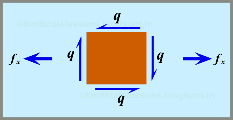
At the NA, there is no stress due to bending, and so, f_x is equal to zero, but q is not equal to zero. In fact, q is maximum at the NA as we saw earlier in the stress distribution (fig.13.5). So for the particles in the NA, the diagram representing the stresses acting on them will be as in fig. 13.7 instead of fig.13.8.

We know that this situation (involving the particle being acted upon only by the shear stress q) is also solved in the text books on 'Strength of Materials'. From those lessons, we know that the plane PQ makes 45^o with the vertical for such a particle. And the stress acting on PQ will have a value numerically equal to q. This is shown in fig.13.13 below:

Fig.13.13 :
Plane PQ of a particle in the NA

The direction of PQ in such a particle is shown in fig.13.14 below:

Fig.13.14 

Direction of plane PQ

Based on the above figs. 13.13 and 13.14, we can easily draw the details of the other principal plane RS. The force on RS will be compressive in nature, and the direction of RS will be perpendicular to PQ. These are shown in figs.13.15 and 13.16 below:

Fig.13.15

Plane RS of a particle in the NA

Fig.13.16

Direction of plane RS, on a particle in the NA

So now we are in a position to calculate the stresses and their directions on any particle in the beam.

Let us consider an actual simply supported beam AB made of a homogeneous material like steel or timber. It's dimensions are shown below in fig.13.17:

Fig.13.17

Simply supported beam

Let this beam carry a udl of 22 kN/m. including self weight.

The reactions at the supports will be: R_A = R_B  = 46.2 kN

The Bending moment at any section along the length of the beam in kNm is given by Eq.13.9: M = 46.2 x - 11 x².

The first differential of this equation will give the equation for SF. Thus:

Eq.13.10: V = 46.2 - 22 x

Where x is the distance of the section measured from support A.

We can consider a number of particles in the body of beam AB, and calculate the stresses and their directions in each of these particles. From Eqs.13.1, 13.5, 13.7 etc.,  we can see that the resultant stress on any particle will depend up on the shear force V and the bending moment M at the section in which the particle is situated. It will also depend on the distance y of the particle from the NA. So we need to know the exact position of the particle in the body of the beam. Let us form a grid as shown in fig.13.18 below:

Fig.13.18

In the above fig., the beam is divided horizontally into 12 equal parts, each of 35 cm width. (35 x 12 = 420 cm). It is also divided vertically into 8 equal parts, each of 5 cm height. (5 x 8 = 40 cm). We are going to take the particles at each 'point of intersection' of the horizontal and vertical grid lines.

We know that, when we consider the vertical grid lines, all particles in any one vertical grid line will be experiencing the same BM, regardless of their vertical distance from the NA. Similarly, all particles in any one vertical grid line will be experiencing the same Shear force V, regardless of their vertical distance from the NA. So we need not consider the horizontal grid lines for the BM and SF. There will be only one unique value for the BM, and another unique value for the SF at a vertical grid line. This is shown in table 13.1 below: (clicking on the figs. will give an enlarged view)

Table 13.1: Values of BM and SF

---

Now we are ready to calculate the stresses. We are analysing the particles at the intersection of the grid lines. As the first step, the stress f_x on each of these particles is calculated using Eq.13.4:

Eq.13.4:

The values are given in table 13.2 below:

Table 13.2 : Values of f_x

Sample calculation:

Let us take the particle at the intersection of Grid 315 and Grid 30.

From table 13.1, M =36.383 KNm.

Distance of this particle from the NA = y = 30 -20 = 10 cm = 0.1 m

Moment of inertia of the whole section =I =bD³/12  = 0.0008 m⁴ 

Substituting these values in Eq.13.4 we get,  f_x = 454.78 kN/m² 

This is equal to 0.455 N/mm².

In the above table, the following points can be noted:

• The values are symmetric about the Grid 210, as this grid line marks the midpoint of the beam

• The values are symmetric about the Grid 20, as this grid line marks the NA. But the values have opposite signs. The values below the NA are positive, indicating Tension, and those above NA are negative, indicating compression.

Next we calculate the stress q on each of the particles using Eq.13.1. We will do it in the next section.

PREVIOUS

NEXT

         

Copyright ©2015 limitstatelessons.blogspot.com - All Rights Reserved

Chapter 13 - Shear stress in beams

Upto the previous section, we were discussing the effects of bending on a beam or slab. When a beam or a slab is loaded, it bends. The beam resists the bending by developing an 'internal moment of resistance'. We discussed about it's details in the previous chapters. We analysed beam and slab sections to determine how much resisting moment they will offer at ultimate state. We designed beam and slab sections in such a way as to make them capable to resist the factored bending moments acting on them.

In addition to the bending moment, shear forces also act on the beam. We have learned about it in the 'Strength of Materials' classes. There we learned to draw shear force diagrams for various loading conditions like concentrated loads, uniformly distributed loads, uniformly varying loads etc., We also learned how to draw the shear force diagrams for the above types of loads, for various support conditions like simply supported, continuous, cantilever support etc., In this chapter we will learn how to make beam and slab sections capable to resist the factored shear forces acting on them. We will also learn how to analyse and determine the 'shear resistance' that a given beam is able to offer at ultimate state. Reinforced concrete beam is a non-homogeneous material consisting of concrete and steel. We will first discuss about the shear forces in a homogeneous material like timber or steel.

Consider a load applied on the beam in fig.13.1. It is made up of a number of wooden planks stacked one above the other.

Fig.13.1:

Beam made up of stacked wooden planks.

The planks are simply stacked, with no bonding between them. When a load is applied, the beam bends. The bending is shown in the animation in fig.13.2 below:

Fig.13.2:

Bending of the stacked planks

Fig.13.3:

Final deflected shape

We can see that there is some horizontal movement for each of the individual planks. That is., the planks slide past each other. So there exists a horizontal force which move the planks in the horizontal direction. If these planks were glued together, then the planks would not have moved horizontally. But then, the glue at the interfaces between the planks will experience a shearing force. Note that the force experienced by the glue is of 'shearing' in nature. It is not 'tensile' or 'compressive'. If it was tensile or compressive, then the planks will be pulling away from each other or pushing onto each other. But here, they are sliding past each other.

In the text books on 'Strength of Materials', a formula is derived for calculating this shear force:

Eq.13.1: q = ^VQ⁄_Ib

The details of this formula are shown in the fig. below:

Fig.13.4:

Horizontal shear acts on any horizontal plane EF

• EF is a horizontal plane at a distance of 'y' from the NA

• V is the Shear force at  the section

• Q is the moment of area (of the portion above EF) about the NA. It can be easily  calculated from the known values D, which is the total depth of the section, b, the width of the section, and y.

• I is the 'moment of inertia' of the section about the NA. For the rectangular section shown in the fig.,

Eq.13.2: I =bD³/12

We also know that this shear stress q have a parabolic distribution across the section. The maximum value will be at the peak of the parabola. It is at the NA, and the value there is 3V/2bD. This is shown in fig.13.5 below:

Fig.13.5:

Horizontal shear stress distribution across the section

So if we take any elementary particle from a beam, except from the top and bottom most fibres, there will be a horizontal shear stress on top and bottom of that particle, as shown in fig.13.6 given below:

Fig.13.6 

Horizontal shear stresses on a particle

But a particle acted upon by the forces shown in fig.13.6 will not be in equilibrium. It will spin. So there will be equal and opposite shear stresses on the vertical sides also. We have learned about this as the principle of 'Complementary shears'. So fig.13.6 can be modified as fig.13.7 given below:

Fig.13.7 

All the shear stresses acting on the particle

But these shear stresses are not the only stresses acting on the particle. We know that when the beam bends due to applied loads, the fibres above the NA will be in compression and the fibres below will be in tension. This stress is in a direction along the length of the beam. That is., it acts horizontally. We can denote it by f_x, and determine it from the basic bending equation:

Eq.13.3

From this we get

Eq.13.4

Where

• M = Bending moment acting on the section,

• y = distance of the particle from the NA, and

• I = Moment of inertia of the section about the NA, given by eq.13.2

So the particle that we consider will experience f_x also, in addition to the above shear stresses, and so the fig.13.7 can be modified again to get fig.13.8 given below:

Fig.13.8 

All the stresses acting on the particle

So now we know all the stresses acting on a particle of the beam. We have to learn about the changes that the particle will be subjected to, due to these stresses. The combined effect of these six stresses shown in fig.13.8 may result in any one of the following:
(i) The particle may be pulled from all directions, and thus it may be split up into two particles, or
(ii) It may be pushed from all directions and thus it may be crushed. 

The result will depend on the relative magnitude of the stresses, and the strength of the material. Some materials have greater tensile strength. Particles of such a material will not fail under a pulling force. Some materials have greater compressive strength. Particles of such a material will not fail under a pushing force. In the next section, we will try to make a mathematical formulation of the effect of the stresses.

PREVIOUS

NEXT

         

Copyright ©2015 limitstatelessons.blogspot.com - All Rights Reserved